vbaで散布図を一括作成

データの入力が終わった！

散布図を作ろう！

系列名を入力…x軸を選択…y軸を選択…

系列名を入力…x軸を選択…

データ100個なんて終わりが見えないよ！！

一括で散布図を作るVBA作ったで

神！！！

前編の「データの一括取り込み」で取り込んだデータを使用して一括で散布図を作成するvbaを簡単に解説します。

前編と後編のコードをまとめて少し便利にしたものをこちらにまとめました。

コンテンツ

使い方

すぐ使いたい方ために、先に使い方を解説します。まずは、以下のコードをvisual basicの標準モジュールにコピーしてください。

全体のコード

Sub 散布図作成()

Dim data_quant As Long
Dim x_cell As Range
Dim y_cell As Range
Dim series_cell As Range
Dim x_axis_r As Long
Dim x_axis_c As Long
Dim y_axis_r As Long
Dim y_axis_c As Long
Dim title As Variant
Dim row_x As Long
Dim row_y As Long


'以下データ入力
    data_quant = Application.InputBox(prompt:="グラフ作成するデータ数を入力してください", _
                                title:="数値入力", _
                                Type:=1)
    If data_quant = False Then
        MsgBox "キャンセルします"
        Exit Sub
    End If
    
    If data_quant > 1 Then
        column_quant = Application.InputBox(prompt:="x軸と次のx軸データの間にある列数を入力してください", _
                                    Default:=column_quant, _
                                    title:="数値入力", _
                                    Type:=1)
        If column_quant = False Then
            MsgBox "キャンセルします"
            Exit Sub
        End If
    Else
    End If
    
    On Error Resume Next
    
    Set x_cell = Application.InputBox(prompt:="一個目のx軸のデータの一個目のセルを選択してください", _
                                title:="セル選択", _
                                Type:=8)
    'キャンセルされた場合はSetがエラーとなる
    If Err.Number = 0 Then
    Else
        MsgBox "キャンセルします"
        Exit Sub
    End If
    
    Set y_cell = Application.InputBox(prompt:="一個目のy軸のデータの一個目のセルを選択してください", _
                                title:="セル選択", _
                                Type:=8)
    'キャンセルされた場合はSetがエラーとなる
    If Err.Number = 0 Then
    Else
        MsgBox "キャンセルします"
        Exit Sub
    End If
    
    Set series_cell = Application.InputBox(prompt:="一個目の系列名のデータを選択してください", _
                                title:="セル選択", _
                                Type:=8)
    'キャンセルされた場合はSetがエラーとなる
    If Err.Number = 0 Then
    Else
        MsgBox "キャンセルします"
        Exit Sub
    End If
    
    title = Application.InputBox(prompt:="グラフタイトルを入力してください", _
                                title:="タイトル", _
                                Type:=2)
    If VarType(title) = vbBoolean Then
        MsgBox "キャンセルします"
        Exit Sub
    Else
    End If
'データ入力終わり
Application.ScreenUpdating = False  '画面切り替えのオフ（動作を軽くします）

Dim ch As Chart
Set ch = ActiveSheet.ChartObjects.Add(10, 0, 400, 300).Chart  'グラフの位置設定
ch.ChartType = xlXYScatterLinesNoMarkers  'グラフの種類（マーカーなし折れ線）


With ch

    .HasTitle = True
    .ChartTitle.Text = title 'タイトル名を入力してください
    
    '.HasLegend = True
    '.Legend.Position = xlLegendPositionBottom  '凡例表示をオンにします
    
End With

x_axis_r = x_cell.Row
x_axis_c = x_cell.Column
y_axis_r = y_cell.Row
y_axis_c = y_cell.Column
series_r = series_cell.Row
series_c = series_cell.Column

For i = 1 To data_quant
    
    row_x = Cells(x_axis_r, x_axis_c + (i - 1) * (column_quant + 1)).End(xlDown).Row
    row_y = Cells(y_axis_r, y_axis_c + (i - 1) * (column_quant + 1)).End(xlDown).Row


    With ch.SeriesCollection.NewSeries
        .XValues = Range(Cells(x_axis_r, x_axis_c + (i - 1) * (column_quant + 1)), Cells(row_x, x_axis_c + (i - 1) * (column_quant + 1)))
        .Values = Range(Cells(y_axis_r, y_axis_c + (i - 1) * (column_quant + 1)), Cells(row_y, y_axis_c + (i - 1) * (column_quant + 1)))
        .Name = Cells(series_r + i - 1, series_c)
        '.Line.ForeColor = i
    End With
    
    'With ActiveSheet.ChartObjects(1).Chart.SeriesCollection(i)
     '   .MarkerStyle = xlNone 'マーカーを非表示
    'End With
    
Next

End Sub

使い方

前編でデータを入力し終わったら、散布図作成のコードを実行します。前編で取り込んだ4県のデータをもとに散布図を作ってみます。

4県の気温グラフを作ってみる

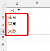
系列名を入力します。入力する場所はどこでも大丈夫です。上から順に入力して下さい。
前編でデータを読み込んだ場合は、A1セルから順にファイル名が入力されているのでそのまま系列名として利用できます。

開発タブ→マクロから「散布図作成」を実行します。データ入力のポップアップが表示されるので以下のように入力していきます。

グラフを作成するデータ数（データ数は、宮城、東京、大阪、沖縄の4県なので、4と入力）
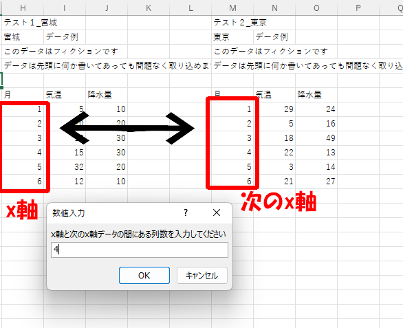
x軸とx軸の間にある列数（今回は、月をx軸とするのでその間の列数4と入力します）
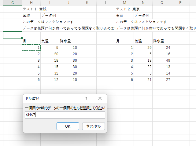
x軸の最初のセルを選択します。データの一番最初のセルを選択します。
y軸の最初のデータのセルも同様に選択
系列名の一個目のデータを選択します。
グラフのタイトルを入力

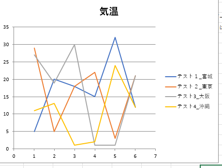
完成！！

各コード解説

1.変数定義

Sub 散布図作成()

Dim data_quant As Long
Dim x_cell As Range
Dim y_cell As Range
Dim series_cell As Range
Dim x_axis_r As Long
Dim x_axis_c As Long
Dim y_axis_r As Long
Dim y_axis_c As Long
Dim title As Variant
Dim row_x As Long
Dim row_y As Long

変数の定義をしています。Longは数値、Rangeはセル範囲、Stringは文字列です。

2.使用するデータ取得

'以下データ入力
    data_quant = Application.InputBox(prompt:="グラフ作成するデータ数を入力してください", _
                                title:="数値入力", _
                                Type:=1)
    If data_quant = False Then
        MsgBox "キャンセルします"
        Exit Sub
    End If
    
    If data_quant > 1 Then
        column_quant = Application.InputBox(prompt:="x軸と次のx軸データの間にある列数を入力してください", _
                                    Default:=column_quant, _
                                    title:="数値入力", _
                                    Type:=1)
        If column_quant = False Then
            MsgBox "キャンセルします"
            Exit Sub
        End If
    Else
    End If
    
    On Error Resume Next
    
    Set x_cell = Application.InputBox(prompt:="一個目のx軸のデータの一個目のセルを選択してください", _
                                title:="セル選択", _
                                Type:=8)
    'キャンセルされた場合はSetがエラーとなる
    If Err.Number = 0 Then
    Else
        MsgBox "キャンセルします"
        Exit Sub
    End If
    
    Set y_cell = Application.InputBox(prompt:="一個目のy軸のデータの一個目のセルを選択してください", _
                                title:="セル選択", _
                                Type:=8)
    'キャンセルされた場合はSetがエラーとなる
    If Err.Number = 0 Then
    Else
        MsgBox "キャンセルします"
        Exit Sub
    End If
    
    Set series_cell = Application.InputBox(prompt:="一個目の系列名のデータを選択してください", _
                                title:="セル選択", _
                                Type:=8)
    'キャンセルされた場合はSetがエラーとなる
    If Err.Number = 0 Then
    Else
        MsgBox "キャンセルします"
        Exit Sub
    End If
    
    title = Application.InputBox(prompt:="グラフタイトルを入力してください", _
                                title:="タイトル", _
                                Type:=2)
    If VarType(title) = vbBoolean Then
        MsgBox "キャンセルします"
        Exit Sub
    Else
    End If
'データ入力終わり

コードを実行するとポップアップが表示されます。ポップアップの設定は、前編で解説したのと同じになります。

変数としてセル範囲持つ場合は、ポップアップの✕ボタンやキャンセルを押した場合の処理が異なります。

3.散布図の設定

Application.ScreenUpdating = False  '画面切り替えのオフ（動作を軽くします）

Dim ch As Chart
Set ch = ActiveSheet.ChartObjects.Add(10, 0, 400, 300).Chart  'グラフの位置設定
ch.ChartType = xlXYScatterLinesNoMarkers  'グラフの種類（マーカーなし折れ線）


With ch

    .HasTitle = True
    .ChartTitle.Text = title 'タイトル名を入力してください
    
    '.HasLegend = True
    '.Legend.Position = xlLegendPositionBottom  '凡例表示をオンにします
    
End With

一行目でマクロ中の画面の切り替えをオフにして動作を軽くしています。

基本的には、コメントの内容を設定しています。グラフの種類を変更したい場合は、「vba グラフ　作り方」などで検索するといいと思います。

グラフなどのオブジェクトを変数に代入するときは、setを使います。

withを使用することでコードを省略するとこができます。今回の場合は、「.HasTitle = True」は実は「ch.HasTitle = True」となっています。

4.散布図の作成

x_axis_r = x_cell.Row
x_axis_c = x_cell.Column
y_axis_r = y_cell.Row
y_axis_c = y_cell.Column
series_r = series_cell.Row
series_c = series_cell.Column

For i = 1 To data_quant
    
    row_x = Cells(x_axis_r, x_axis_c + (i - 1) * (column_quant + 1)).End(xlDown).Row
    row_y = Cells(y_axis_r, y_axis_c + (i - 1) * (column_quant + 1)).End(xlDown).Row


    With ch.SeriesCollection.NewSeries
        .XValues = Range(Cells(x_axis_r, x_axis_c + (i - 1) * (column_quant + 1)), Cells(row_x, x_axis_c + (i - 1) * (column_quant + 1)))
        .Values = Range(Cells(y_axis_r, y_axis_c + (i - 1) * (column_quant + 1)), Cells(row_y, y_axis_c + (i - 1) * (column_quant + 1)))
        .Name = Cells(series_r + i - 1, series_c)
        '.Line.ForeColor = i
    End With
    
    'With ActiveSheet.ChartObjects(1).Chart.SeriesCollection(i)
     '   .MarkerStyle = xlNone 'マーカーを非表示
    'End With
    
Next

End Sub

ポップアップで入力したデータをもとに散布図のデータを追加していきます。

入力されたx軸とy軸の一番最初のセルから1つ目の散布図のデータを作成し、データの最大列数から次のデータの位置を計算します。この動作をデータの数分、繰り返して散布図を作成します。系列名は、系列名の選択セルから順に参照します。